Optimizer Baselines
Evaluating optimizers is notoriously difficult as optimizer performance varies greatly across different tasks, and which hyper parameters are used. Never the less, when training learned optimizers, we needed to evaluate them! To that end, we have built, a system as well as a large set of baseline of precomputed optimizers on a variety of tasks.
Distribution of Tasks
We define a set of “fixed” tasks which are functions which produce Task instances and which we evaluate performance of optimizers on. These tasks are named with the same name as the function. For example `ImageMLP_Cifar10_8_Relu32<https://github.com/google/learned_optimization/blob/09a830f098eb372fc7ddfc147289386442347d06/learned_optimization/tasks/fixed/image_mlp.py#L111I>`_ is a task which involves training a tiny MLP. The code for all tasks can be found at learned_optimization/tasks/fixed. Each Task defines a dataset, a batchsize, a loss function and a model architecture. See (Tasks for full info.)
Hyper Parameter Sets
Given one of these tasks we can evaluate some set of baseline optimizers on it. These sets are defined in `learned_optimization/baselines/hparam_sets.py<https://github.com/google/earned_optimization/blob/main/learned_optimization/baselines/hparam_sets.py>`_ and define a list of gin configurations as well as paths with which to save results to.
There are numerous different baselines, each of which defines hyper parameters for the optimizer, (e.g. learning rates), number of random seeds, and details about how frequently to perform evaluations over the course of training.
Training one task
To evaluate an hparam set, one needs to evaluates each configuration. These configurations get passed into an inner-training script `learned_optimization/baselines/run_trainer.py<https://github.com/google/learned_optimization/blob/main/learned_optimization/baselines/run_trainer.py>`_ which then write out the results.
We release a folder with a large number of evaluations at gs://gresearch/learned_optimization/opt_curves/. To run your own, by default, these will be located at the environment variable LOPT_BASELINE_DIR, or ~/lopt_baselines by default. Each individual run gets stored in a nested folder.
The raw files are in numpy’s savez format, and can be loaded back.
import tensorflow as tf
import numpy as np
path = "gs://gresearch/learned_optimization/opt_curves/MLPMixer_ImageNet64_small16/Yogi_lr1e-05/10000_10_5_10/20220430_001348_8b9b03eb-b.curves"
data ={k:v for k,v in np.load(tf.io.gfile.GFile(path, "rb")).items()}
Or you can leverage learned_optimization.baselines.utils.load_baseline_results_from_dir which globs the directory, and loads all training curves.
Results from multiple trials: Archives
Often times we seek to look at results from multiple trials though. The AdamLR_10000_R5 hparam set, for example, runs 14 learning rates, with 5 random seeds each meaning 70 trials. As these results are useful together, we provide utils to aggregate these 70 files into a single file. These archives are created by `learned_optimization/baselines/run_archive.py<https://github.com/google/learned_optimization/blob/main/learned_optimization/baselines/run_archive.py>`_ which is again configured by gin. which then write out the results.
By default these are stored in the LOPT_BASELINE_ARCHIVES_DIR environment variable, or ~/lopt_baselines_archives. We also provide a set of baselines for many tasks in gs://gresearch/learned_optimization/opt_archives/.
As before, these are simply numpy savez files, and can be loaded directly or with learned_optimization.baselines.load_archive which takes a task name and a hparam set name.
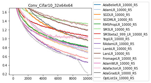
Visualization of results
For ease of access, we have a simple function to visualize multiple different optimizers on a given task. This function loads all the hparam sets, finds the best hyper parameter configuration across the set, performs averages over the different random seeds, and then plots.
from learned_optimization.baselines import vis
opt_sets = [
            "AdaBeliefLR_10000_R5",
            "AdamLR_10000_R5",
            "SGDLR_10000_R5",
            "SGDMLR_10000_R5",
            "RMSPropLR_10000_R5",
            "SM3LR_10000_R5",
            "SM3beta2_999_LR_10000_R5",
            "YogiLR_10000_R5",
            "RAdamLR_10000_R5",
            "LambLR_10000_R5",
            "LarsLR_10000_R5",
            "FromageLR_10000_R5",
            "AdamWLR_10000_R5",
            "AdafactorLR_10000_R5",
            "AdaGradLR_10000_R5",
            "OptList1k_10000_R5",
]

task_name = "Conv_Cifar10_32x64x64"
vis.plot_tasks_and_sets(task_name, opt_sets, alpha_on_confidence=0.0)
Normalization of losses
One cannot directly aggregate performance / loss values across all the different tasks as the loss values mean different things (e.g. cross entropy loss vs mean square error). Nevertheless, understanding aggregate performance is useful when evaluating optimizers. As a solution to this, we have developed loss normalizers which can be used to normalize all losses to the same scales. These normalizers themselves are based on performance measurements from different baselines. See learned_optimization/baselines/normalizers.py for more info.